Create The Journal and Journal Entry with Excel (Part 2)
In part 1, you have study how to create a current date and dropdown list of posting reference identifying the number of the account posted. Now we will study how to link Account Tittle column with Posting Reference column. If you are beginner in excel, maybe you will need more times to practice this method.
 I will show you how to use VLOOKUP function,based on excel help, VLOOKUP is is a function to Search for a value in the first column of a table array and returns a value in the same row from another column in the table array. OK lets start to begin.
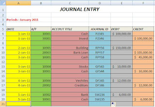
1. Open your last project about….. and select a cell below Account Tittle (ie. The first row on account tittle column). Then type or copy this formula :
=VLOOKUP(B6,TABLE,3,TRUE)
Explanation : B6 is a cell name refers to the first cell on Posting Reference (R/F) column, in this example, the first cell below R/F is B6, so must adjust this function based on yours.
2. Copy down this formula as much as you want, but when you do this, you will see that all the cell will show “#N/A”. Don’t worry, it’s mean that there are no value at PR column. It will automatically filled after you change that value. You can delete it if you want to fill blank cell.
3. Type your Journal ID Number at “Journal ID “ Column. The Journal ID is a your transaction number.
4. Select Debit and Credit Column, change the format cell to Accounting, you can set the Accounting Format from Menu Home -> at format cell dropdown list, select Accounting.
5. To minimalize the mistake from typing a text (debit and credit column receive Number only), you can make Data Validation from Data – Data Validation.Activesettings tab and select Allow: Whole Number, choose Data:Greater than, Minimum : 0. This methods mean that the cell only receive number greater than zero, the text or negative value will unacceptable.

6. To make a warning text, select Error Allert tab. Type at Title: Data Validation, Error Message :"Please Enter Number Greater than 0".

 I will show you how to use VLOOKUP function,based on excel help, VLOOKUP is is a function to Search for a value in the first column of a table array and returns a value in the same row from another column in the table array. OK lets start to begin.
1. Open your last project about….. and select a cell below Account Tittle (ie. The first row on account tittle column). Then type or copy this formula :
=VLOOKUP(B6,TABLE,3,TRUE)
Explanation : B6 is a cell name refers to the first cell on Posting Reference (R/F) column, in this example, the first cell below R/F is B6, so must adjust this function based on yours.
2. Copy down this formula as much as you want, but when you do this, you will see that all the cell will show “#N/A”. Don’t worry, it’s mean that there are no value at PR column. It will automatically filled after you change that value. You can delete it if you want to fill blank cell.
3. Type your Journal ID Number at “Journal ID “ Column. The Journal ID is a your transaction number.
4. Select Debit and Credit Column, change the format cell to Accounting, you can set the Accounting Format from Menu Home -> at format cell dropdown list, select Accounting.
5. To minimalize the mistake from typing a text (debit and credit column receive Number only), you can make Data Validation from Data – Data Validation.Activesettings tab and select Allow: Whole Number, choose Data:Greater than, Minimum : 0. This methods mean that the cell only receive number greater than zero, the text or negative value will unacceptable.

6. To make a warning text, select Error Allert tab. Type at Title: Data Validation, Error Message :"Please Enter Number Greater than 0".


Comments